Quanser Aero PID Control Design | Anuranan Bharadwaj

Role

Team Member — PID Tuning & System Identification

AE 443: Experimental Dynamics & Control · ERAU · Spring 2026

Tools

MATLAB · Simulink · QUARC Real-Time Control
Transfer Function Analysis · Bode / Frequency Response

Key Contributions

Tuned PID controller (k_p = 8, k_d = 3.1, k_i = 5) achieving 4.12% overshoot against a sub-16.7% design spec
Identified second-order plant model from experimental step response: ζ = 0.0452, ω_n = 2.18 rad/s
Derived analytical PID gains from pole-placement and verified phase margin improvement from 3.68° to 87.5°
Compared model-based and manually tuned controllers, demonstrating why empirical tuning outperformed the analytical design for tracking a square-wave command

This page walks through the pitch-axis control design for the Quanser Aero lab platform — from characterizing the open-loop dynamics, through individually tuning each PID term, to deriving an analytical second-order model and comparing it against the empirically tuned controller.

System Description & Objectives

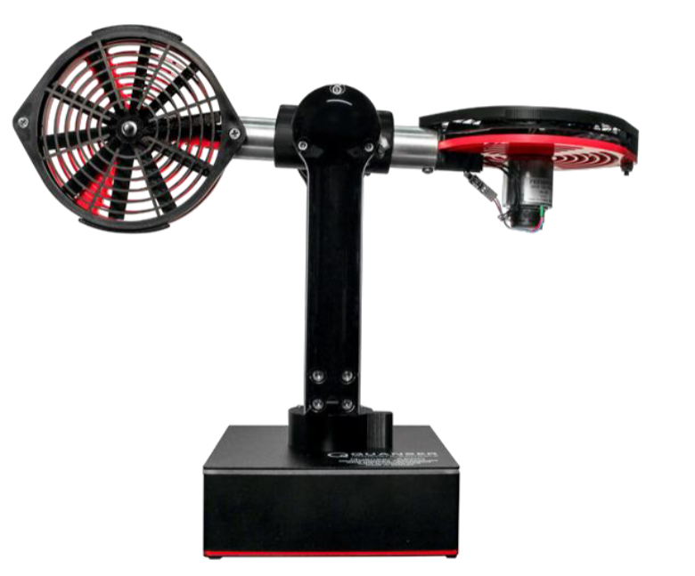
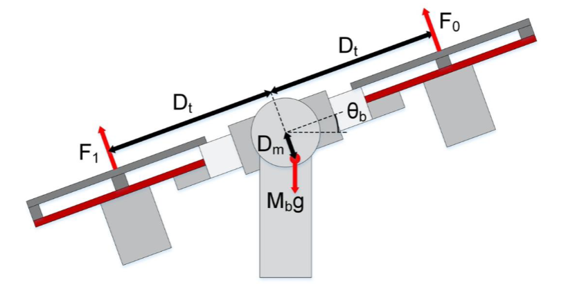
The Quanser Aero is a two-degree-of-freedom laboratory platform that mimics the pitch and yaw dynamics of a helicopter body. Two brushless DC motors drive propellers mounted at the ends of a rigid arm; the resulting thrust forces create moments about the pitch axis (elevation) and the yaw axis (travel). The platform is instrumented with encoders on both axes and connects to a host PC through QUARC real-time software, which closes the control loop in hardware at millisecond sampling rates. Because the aerodynamic coupling, inertia, and motor dynamics are all present, the Quanser Aero provides a physically meaningful testbed for classic control techniques well beyond pure simulation.

This project focused exclusively on the pitch axis. The objectives were:

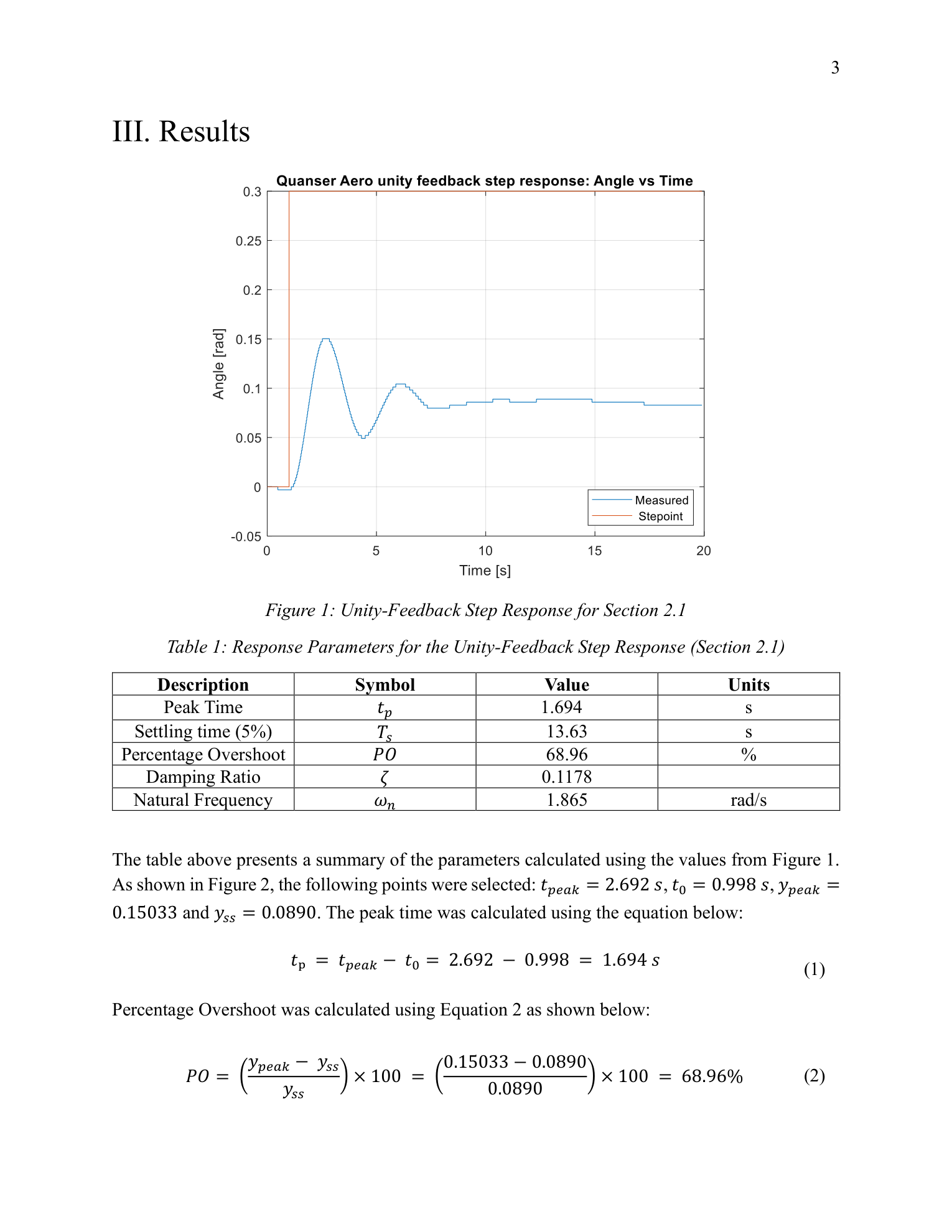
Characterize the open-loop pitch response and extract key transient parameters (ω_n, ζ, settling time)
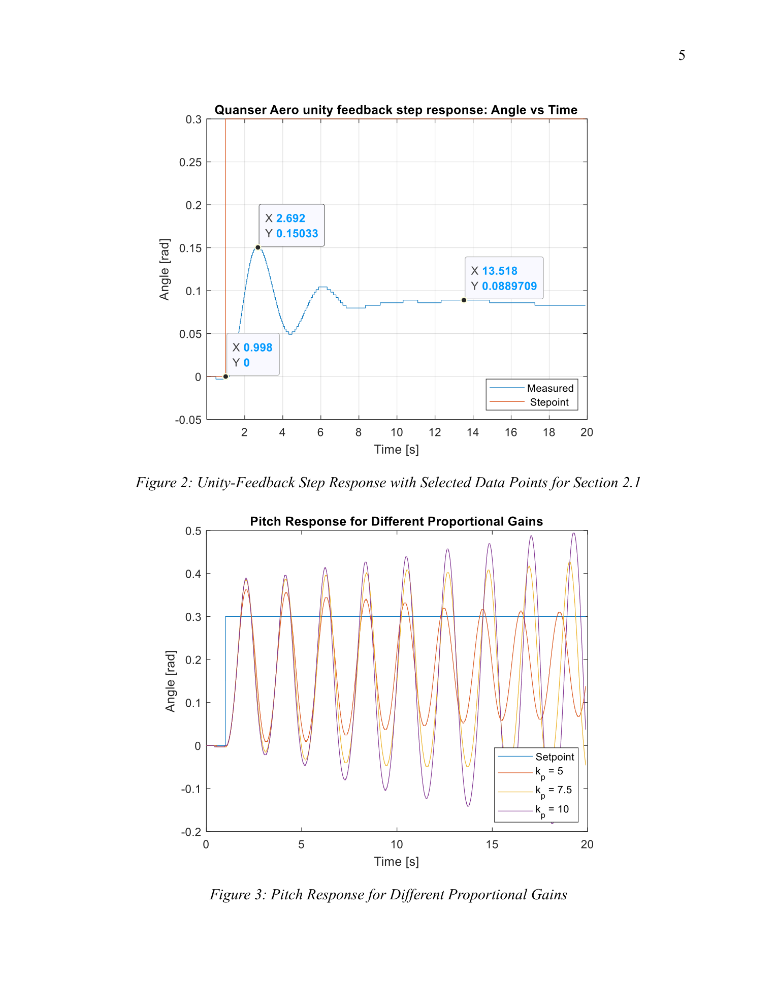
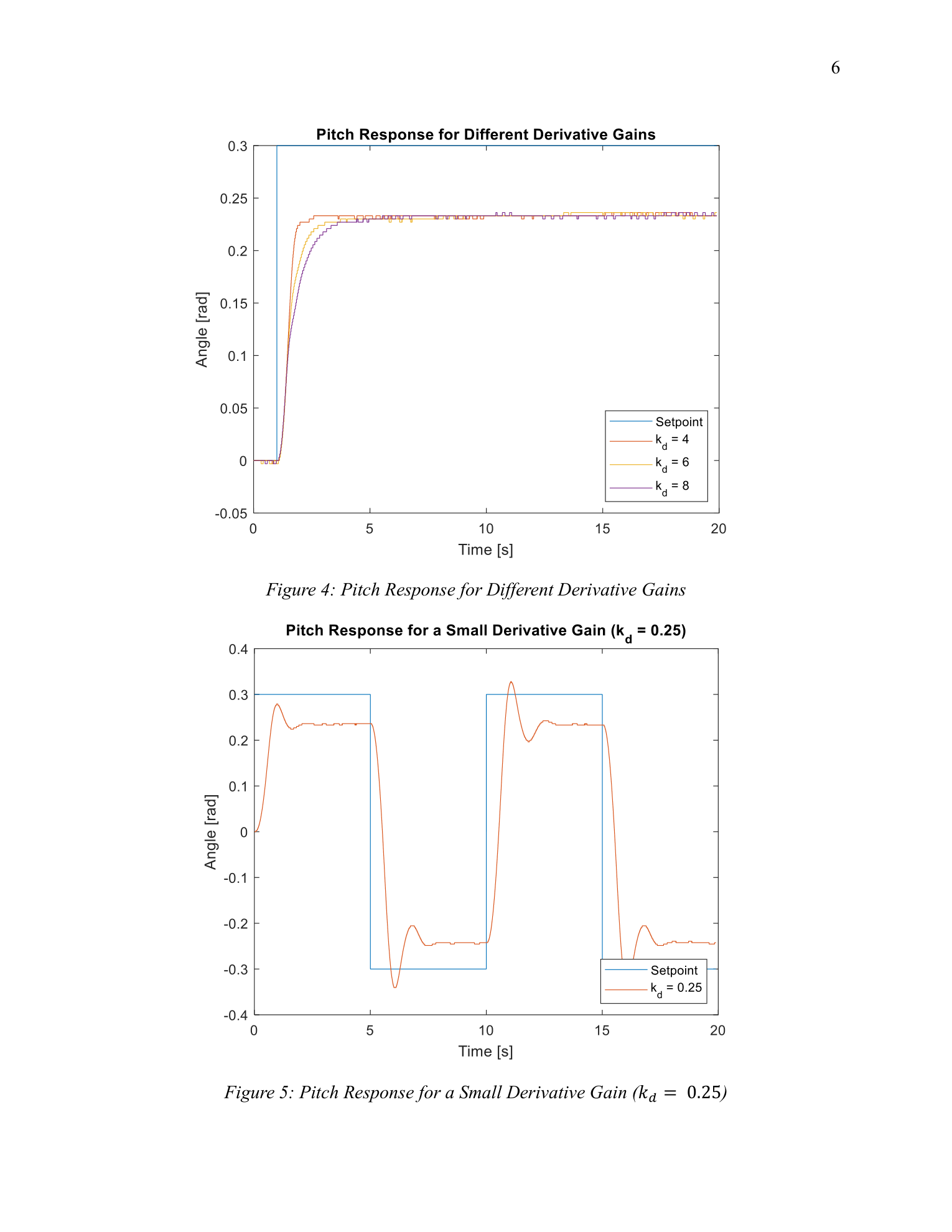
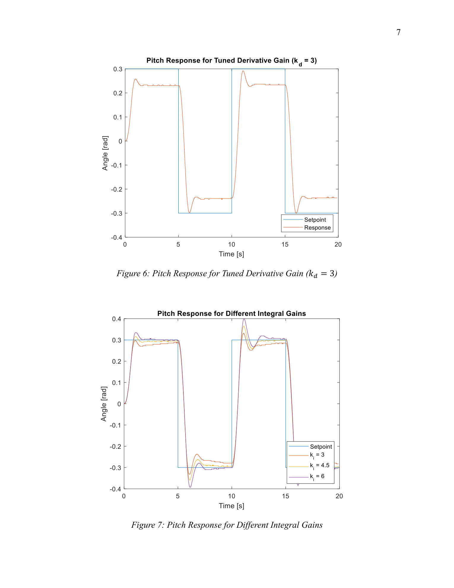
Systematically study the individual effects of proportional, derivative, and integral control action on response speed, damping, and steady-state error
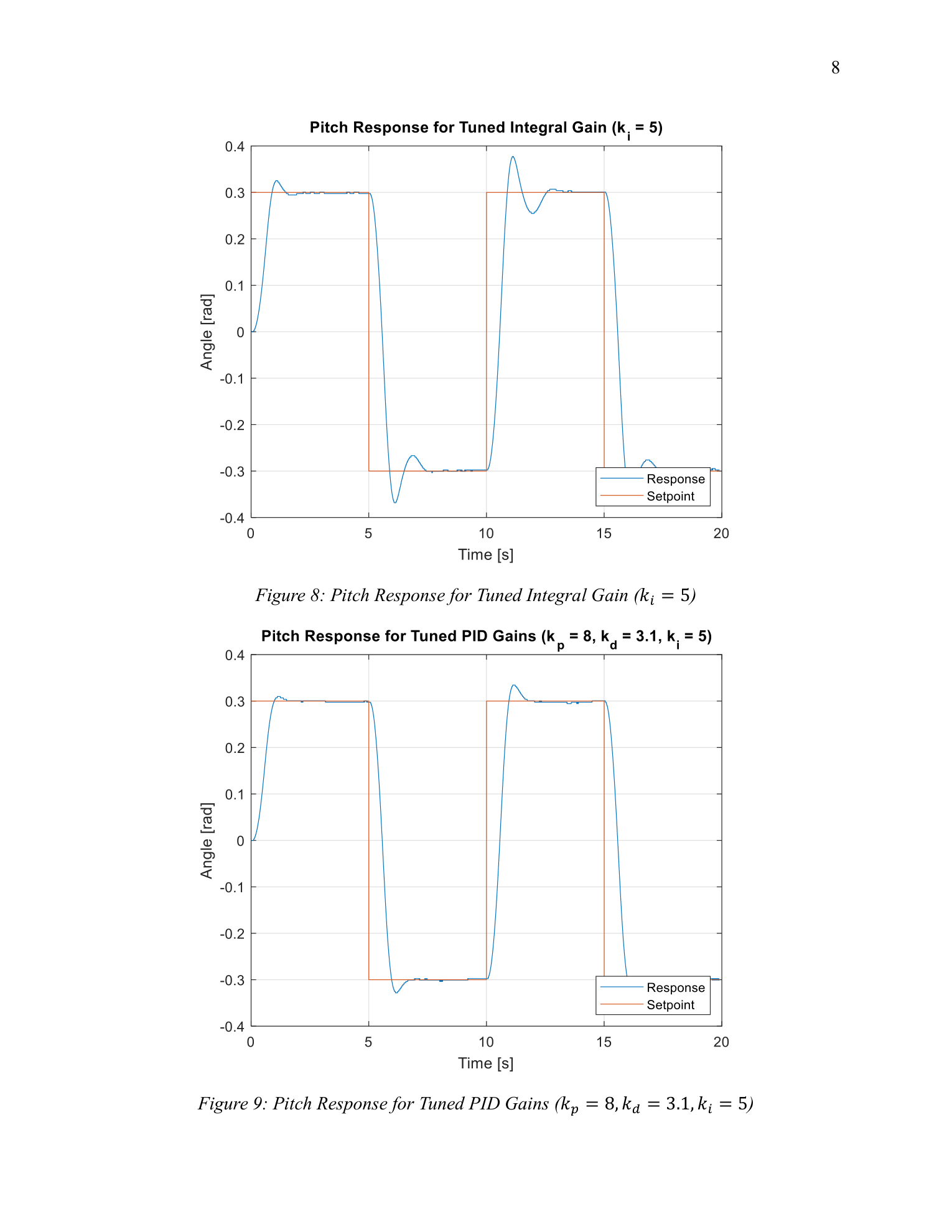
Tune a PID controller to meet design requirements: peak pitch ≤ 0.35 rad and peak time < 1.1 s for a 0.3 rad square-wave command
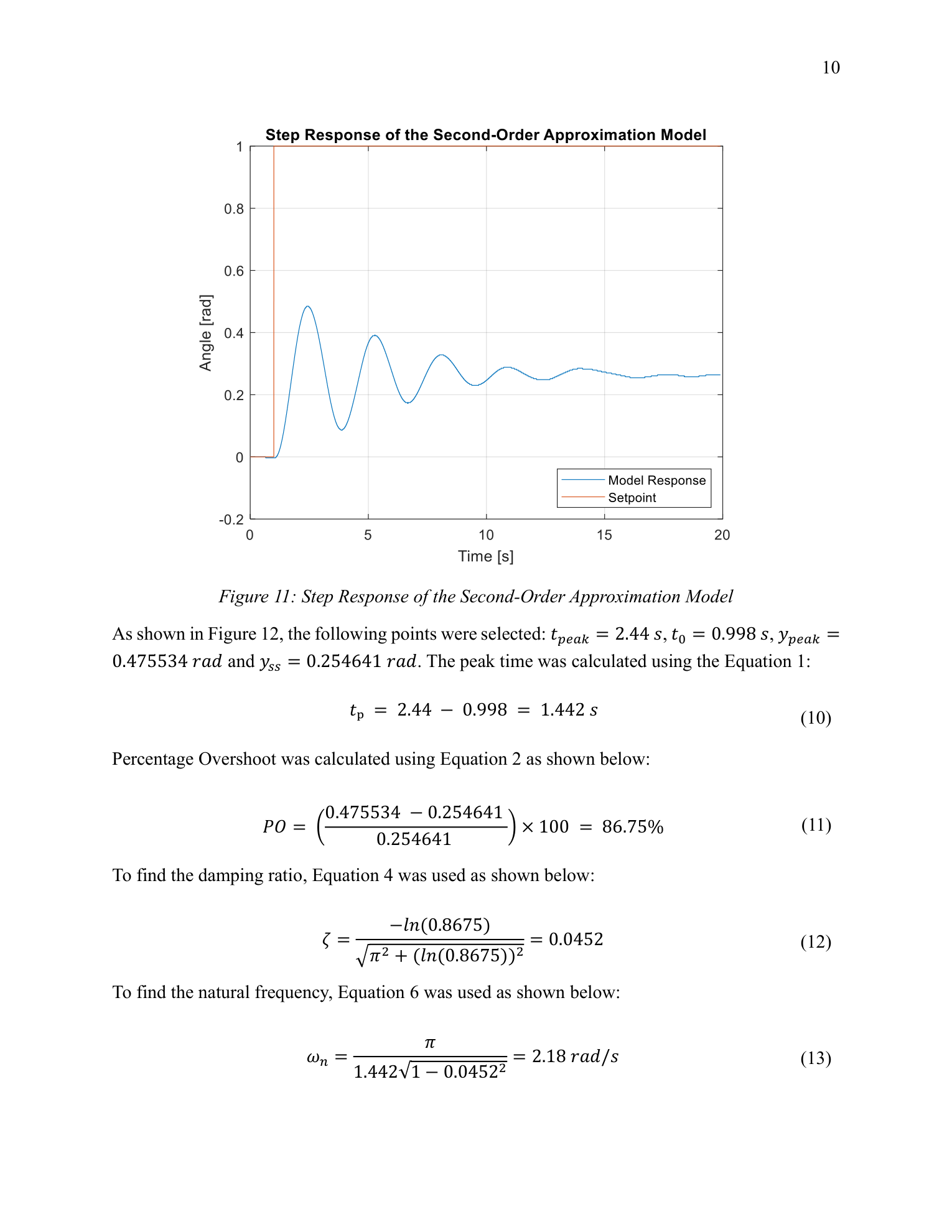
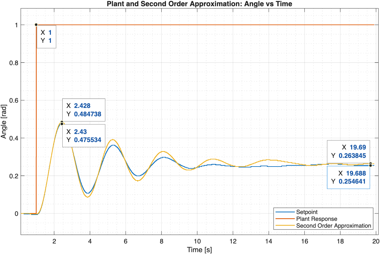
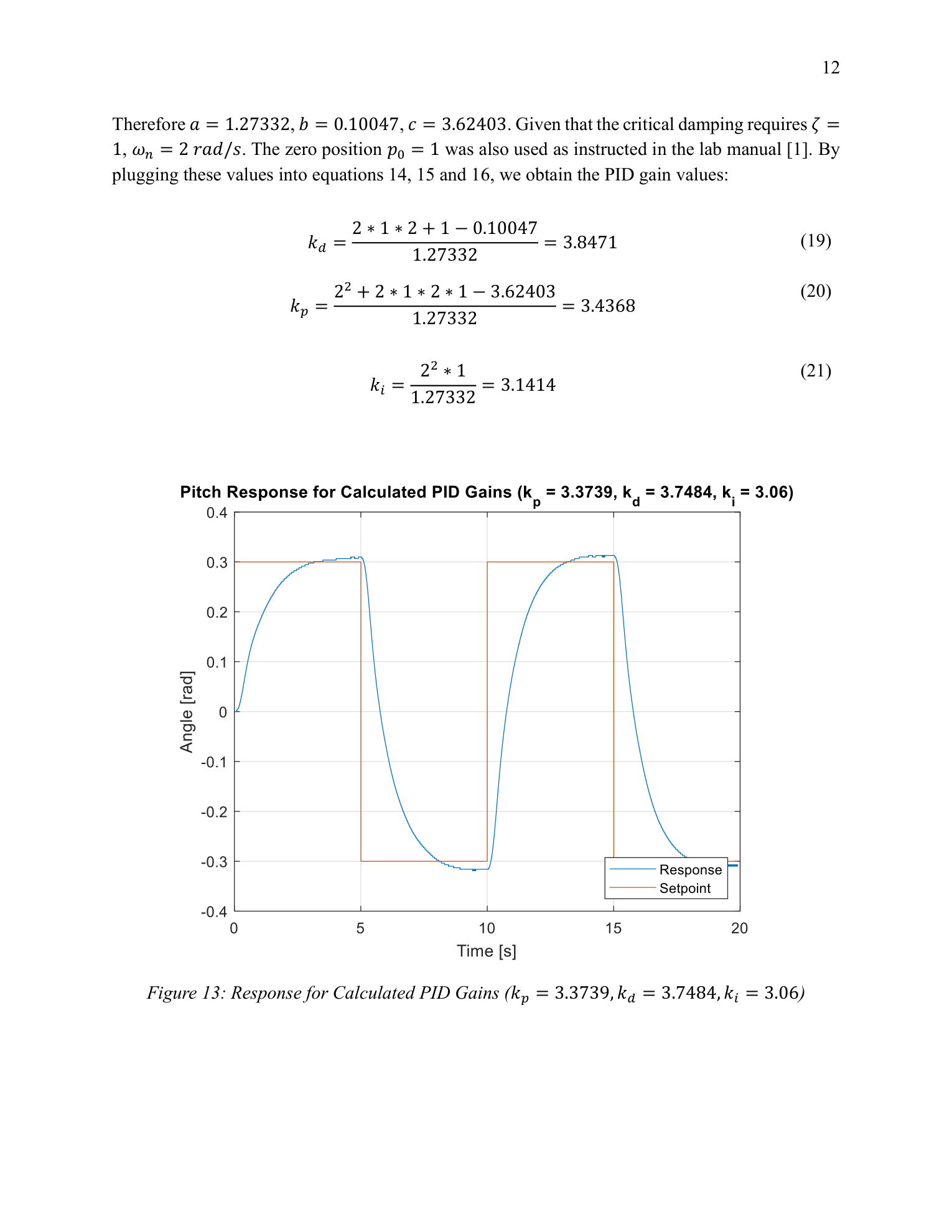
Develop a second-order plant model from experimental data and use it to calculate PID gains analytically, then compare with the tuned controller
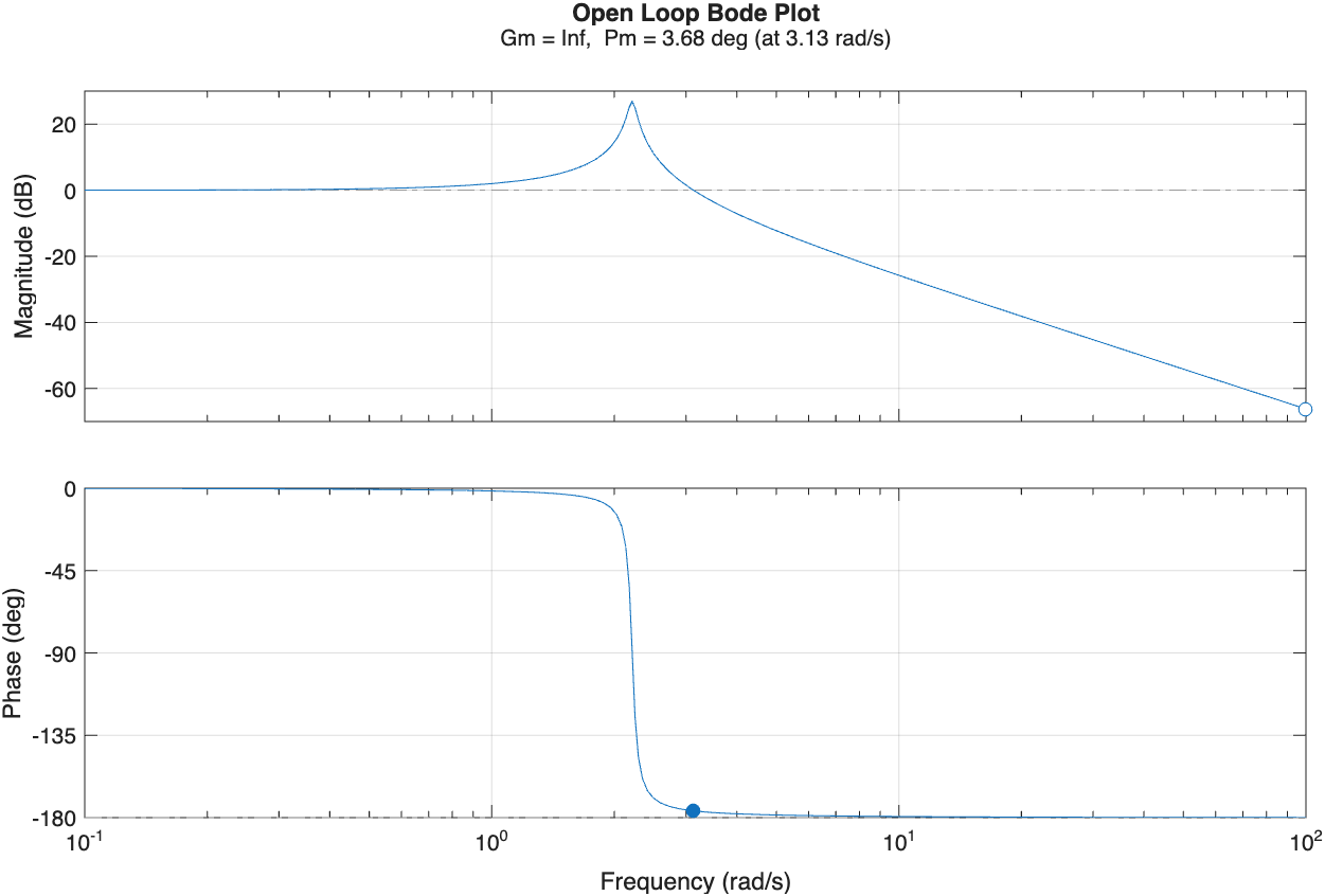
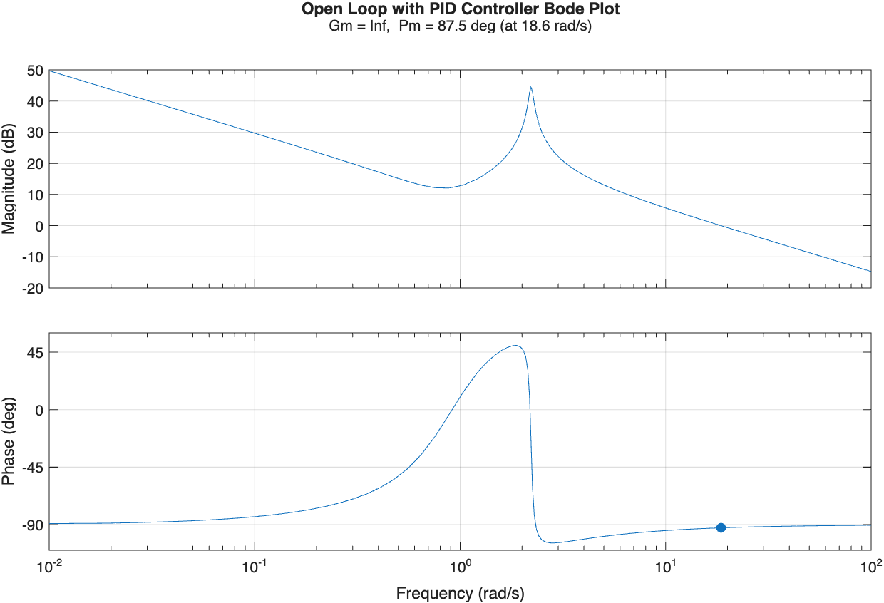
Evaluate closed-loop stability margins using Bode analysis in MATLAB

Quanser Aero hardware setup — Fig. 1: Quanser Aero Setup — two brushless DC motors driving propellers mounted on a rigid arm, instrumented for pitch and yaw control

Free body diagram of Quanser Aero — Fig. 2: Free Body Diagram of Quanser Aero — thrust forces F₀, F₁ at distance D_t, body mass M_bg at offset D_m, pitch angle θ_b

Open-Loop System Characterization

The experiment began with a unity-feedback step response on the uncompensated pitch axis to measure baseline dynamics. From the measured response, the following key points were identified:

t_peak = 2.692 s · t₀ = 0.998 s (step onset) · y_peak = 0.15033 rad · y_ss = 0.0890 rad

These values were used to compute the standard second-order metrics:

Parameter	Symbol	Value
Peak Time	t_p	1.694 s
Settling Time (5%)	T_s	13.63 s
Percentage Overshoot	PO	68.96%
Damping Ratio	ζ	0.1178
Natural Frequency	ω_n	1.865 rad/s

With a damping ratio of ζ = 0.1178, the uncompensated Quanser Aero pitch axis is highly underdamped. The 68.96% overshoot and 13.63-second settling time confirm that compensation is required before the platform can track any meaningful command.

Unity-feedback open-loop step response of Quanser Aero pitch axis — Fig. 3 & Table 1: Unity-feedback open-loop step response — PO = 68.96%, T_s = 13.63 s, ω_n = 1.865 rad/s

Effect of Each Control Action on Pitch Response

Proportional Gain

Proportional gain k_p was varied from 5 to 10 in steps of 2.5.

Increasing k_p decreased peak time only slightly — from ~1.17 s at k_p = 5 to ~1.1 s at k_p = 10
Percentage overshoot grew sharply, from ~20% up past 60%, with oscillations that failed to decay at the highest gain

Proportional control alone could not satisfy both the peak time and overshoot requirements simultaneously.

Pitch response for three proportional gains — Fig. 4: Pitch response for k_p ∈ {5, 7.5, 10} — faster response but rapidly growing overshoot

Derivative Gain

Derivative gain k_d was varied from 4 to 8 in steps of 2, with k_p held fixed.

All three values produced zero percent overshoot — a significant improvement
The tradeoff was increasing peak time, from ~1.6 s at k_d = 4 to ~2.6 s at k_d = 8
A secondary test at k_d = 0.25 showed the expected fast but oscillatory response, confirming the damping role of the derivative term

Pitch response for three derivative gains — Fig. 5 & 6: Pitch response for k_d ∈ {4, 6, 8} and k_d = 0.25 — derivative action eliminates overshoot but slows response

Integral Gain

With the square-wave input active, integral gain k_i was varied from 3 to 6 in steps of 1.5.

At k_i = 3, the system tracked below the setpoint
At k_i = 6, steady-state error was nearly eliminated, but overshoot grew to ~0.4 rad and inter-cycle oscillations became pronounced
A tuned value of k_i = 5 gave a steady-state pitch of 0.2976 rad (setpoint: 0.3 rad) with controlled overshoot

Pitch response for tuned derivative gain and integral gain sweep — Fig. 7 & 8: Tuned derivative gain (k_d = 3, y_peak = 0.2577 rad) and integral gain sweep (k_i ∈ {3, 4.5, 6})

Final PID Tuning & Performance

The three gains were tuned simultaneously on the hardware until the combined response met all design requirements. The final tuned gains were k_p = 8, k_d = 3.1, k_i = 5. These values were chosen by first setting k_p high enough for fast rise, then adding k_d to suppress oscillations, and finally increasing k_i incrementally to drive out the remaining steady-state error without reintroducing instability.

Parameter	Value	Specification	Met?
Peak Time (t_p)	1.18 s	< 1.1 s	✗ (marginal)
Percentage Overshoot	4.12%	Peak ≤ 0.35 rad	✓
Steady-State Value	0.2976 rad	~0.3 rad	✓

Pitch response with final tuned PID gains — Fig. 9 & 10: Tuned k_i = 5 response (left) and final PID k_p = 8, k_d = 3.1, k_i = 5 square-wave tracking (right) — 4.12% overshoot, y_ss = 0.2976 rad

Second-Order System Identification & Analytical PID Design

A second independent step response was recorded under unity feedback to derive a second-order plant model. From the measured data (y_peak = 0.4755 rad, y_ss = 0.2546 rad, t_p = 1.442 s), the following model parameters were calculated:

Percentage Overshoot: 86.75%
Damping Ratio: ζ = 0.0452
Natural Frequency: ω_n = 2.18 rad/s

The resulting second-order transfer function approximating the Quanser Aero pitch axis is:

G(s) = 1.27332 / (s² + 0.10047s + 3.62403)

To validate the model, its simulated step response was overlaid with the experimental plant response. The agreement was strong: peak time error was only 0.14%, percent overshoot error was 3.48%, and steady-state difference was 3.61%. The small errors confirm the approximation captures the dominant dynamics well, though higher-order effects (friction, actuator saturation) prevent a perfect match.

Step response of second-order approximation model — Fig. 11: Simulated step response of the identified second-order model — captures peak time and overshoot within 3.5%

Combined comparison of plant and second-order model responses — Fig. 12: Overlaid plant (hardware) and second-order model responses — steady-state error between responses is 0.0092 rad (3.61%)

Analytically Calculated PID Gains

Using the identified transfer function coefficients (a = 1.27332, b = 0.10047, c = 3.62403) and a target of critically damped response (ζ_d = 1, ω_nd = 2 rad/s) with integrator zero p₀ = 1, the three PID gains were solved analytically:

k_d = (2ζ_dω_nd + p₀ − b) / a = 3.847
k_p = (ω_nd² + 2ζ_dω_ndp₀ − c) / a = 3.437
k_i = ω_nd²p₀ / a = 3.141

For hardware testing, the workbook solution values (k_p = 3.3739, k_d = 3.7484, k_i = 3.06) were used. These produced a critically damped square-wave response with 0% overshoot and a peak time of 4.64 s — considerably slower than the tuned controller due to the conservative critical damping target and the limitations of the second-order approximation.

Design Decision

Trade-off: The analytically derived gains targeted a critically damped response, producing 0% overshoot but a peak time of 4.64 s — nearly four times slower than the empirically tuned controller's 1.18 s.

Why: The conservative critical-damping target, combined with the second-order model's limitations (it does not capture friction or actuator saturation), made the analytical gains too sluggish for square-wave tracking. Empirical tuning of k_p = 8, k_d = 3.1, k_i = 5 on the actual hardware compensated for these unmodeled effects and met the speed requirement directly.

Pitch response using analytically calculated PID gains — Fig. 13: Square-wave response using calculated PID gains (k_p = 3.3739, k_d = 3.7484, k_i = 3.06) — 0% overshoot but sluggish tracking

Frequency-Domain Analysis & Stability Margins

Bode plots were generated in MATLAB for both the open-loop plant and the PID-compensated open loop. The plant transfer function G(s) = ω_n² / (s² + 2ζω_ns + ω_n²) was combined with the PID controller C(s) = k_p + k_i/s + k_ds, and the margin() function was used to extract gain margins, phase margins, and bandwidth.

System	Phase Margin	Gain Margin	Bandwidth
Open Loop (plant only)	3.68°	∞	N/A
PID Compensated	87.5°	∞	19.32 rad/s

The open-loop plant has a phase margin of only 3.68°, placing it right at the edge of instability — consistent with the severe oscillations seen in the open-loop step response. Adding the PID controller drives the phase margin to 87.5°, a dramatic improvement indicating robust stability with ample damping. The gain margin is infinite for both cases because the phase never crosses −180° in the frequency range of interest.

Open-loop Bode plot of Quanser Aero plant — Fig. 14: Open-loop Bode plot — phase margin = 3.68°, barely stable; gain margin = ∞

Bode plot of PID-compensated open loop — Fig. 15: PID-compensated open-loop Bode plot — phase margin improved to 87.5°, bandwidth = 19.32 rad/s

State-Space Formulation & System Properties

The identified second-order transfer function was converted to state-space form by defining states x₁ = y (pitch angle) and x₂ = ˙y (pitch rate). The resulting matrices are:

A = [[0, 1], [−ω_n², −2ζω_n]] B = [[0], [ω_n²]] C = [1, 0] D = [0]

The controllability matrix P_c has determinant −ω_n⁴ ≠ 0 and rank 2, confirming the system is fully controllable. The observability matrix P_o = I_2×2, so det(P_o) = 1 and rank = 2, confirming full observability. Although the system satisfies the necessary conditions for state-feedback control, PID remains the more practical choice here: the plant is simple enough that the additional complexity of a full state observer is not justified.

Key Takeaways

Manual tuning outperformed model-based design for tracking a square-wave command.

The analytically calculated gains produced 0% overshoot but tracked the command too slowly (t_p = 4.64 s vs. 1.18 s for the tuned controller). The second-order model was adequate for linear analysis but missed friction, actuator limits, and higher-order dynamics that empirical tuning naturally compensated for.

PID compensation transformed a nearly unstable plant into a robustly stable closed loop.

The open-loop Quanser Aero pitch axis had a phase margin of only 3.68° — one small perturbation from instability. Adding the PID controller raised the phase margin to 87.5°, transforming a poorly damped (ζ = 0.0452) system into one with reliable, repeatable square-wave tracking.

Each gain has a distinct, quantifiable trade-off between speed and stability.

Increasing k_p alone pushed overshoot past 60%; increasing k_d alone pushed peak time past 2.6 s; increasing k_i alone caused oscillations at the square-wave transitions. The final tuned combination (k_p = 8, k_d = 3.1, k_i = 5) balanced all three effects to satisfy both speed and damping requirements simultaneously.

A second-order step-response model can capture dominant dynamics with <4% error.

The identified transfer function G(s) = 1.27332 / (s² + 0.10047s + 3.62403) reproduced the hardware step response with 0.14% peak-time error and 3.48% overshoot error. This validates the second-order approximation method as a fast, practical tool for controller pre-design, even when the real plant contains unmodeled nonlinearities.